2020 US Election Results vs Vaccination
Introduction
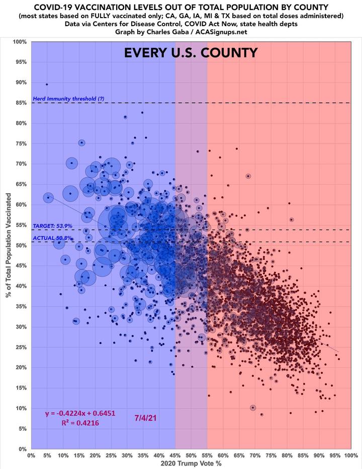
The purpose of this exercise is to reproduce a plot using your dplyr and ggplot2 skills. Read the article The Racial Factor: There’s 77 Counties Which Are Deep Blue But Also Low-Vaxx. Guess What They Have In Common? and have a look at the above figure.
Datasets that are going to be used for the exercise.
- To get vaccination by county, we will use data from the CDC
- You need to get County Presidential Election Returns 2000-2020
- Finally, you also need an estimate of the population of each county
# Download CDC vaccination by county
cdc_url <- "https://data.cdc.gov/api/views/8xkx-amqh/rows.csv?accessType=DOWNLOAD"
vaccinations <- vroom(cdc_url) %>%
  janitor::clean_names() %>%
  filter(fips != "UNK") # remove counties that have an unknown (UNK) FIPS code

# Download County Presidential Election Returns
# https://dataverse.harvard.edu/dataset.xhtml?persistentId=doi:10.7910/DVN/VOQCHQ -- Download the file from the given URL into your base repository
election2020_results <- vroom(here::here("csv", "countypres_2000-2020.csv")) %>% #read the file from the location you saved it to
  janitor::clean_names() %>%

  # just keep the results for the 2020 election
  filter(year == "2020") %>%

  # change original name county_fips to fips, to be consistent with the other two files
  rename (fips = county_fips)

# Download county population data
population_url <- "https://www.ers.usda.gov/webdocs/DataFiles/48747/PopulationEstimates.csv?v=2232"
population <- vroom(population_url) %>%
  janitor::clean_names() %>%

  # select the latest data, namely 2019
  select(fips = fip_stxt, pop_estimate_2019) %>%

  # pad FIPS codes with leading zeros, so they are always made up of 5 characters
  mutate(fips = stringi::stri_pad_left(fips, width=5, pad = "0"))
Explore the Data
A quick look at the columns within each dataframe tells us which variables we need to filter for later on to build the graph.
head(election2020_results)## # A tibble: 6 × 12
## year state state_po county_name fips office candidate party candidatevotes
## <dbl> <chr> <chr> <chr> <chr> <chr> <chr> <chr> <dbl>
## 1 2020 ALABAMA AL AUTAUGA 01001 PRESIDENT JOSEPH R… DEMO… 7503
## 2 2020 ALABAMA AL AUTAUGA 01001 PRESIDENT OTHER OTHER 429
## 3 2020 ALABAMA AL AUTAUGA 01001 PRESIDENT DONALD J… REPU… 19838
## 4 2020 ALABAMA AL BALDWIN 01003 PRESIDENT JOSEPH R… DEMO… 24578
## 5 2020 ALABAMA AL BALDWIN 01003 PRESIDENT OTHER OTHER 1557
## 6 2020 ALABAMA AL BALDWIN 01003 PRESIDENT DONALD J… REPU… 83544
## # … with 3 more variables: totalvotes <dbl>, version <dbl>, mode <chr>head(population)## # A tibble: 6 × 2
## fips pop_estimate_2019
## <chr> <dbl>
## 1 00000 328239523
## 2 01000 4903185
## 3 01001 55869
## 4 01003 223234
## 5 01005 24686
## 6 01007 22394head(vaccinations)## # A tibble: 6 × 27
## date fips mmwr_week recip_county recip_state series_complete_pop_…
## <chr> <chr> <dbl> <chr> <chr> <dbl>
## 1 09/14/2021 05073 37 Lafayette County AR 31.2
## 2 09/14/2021 35047 37 San Miguel County NM 42.8
## 3 09/14/2021 37159 37 Rowan County NC 35.1
## 4 09/14/2021 16021 37 Boundary County ID 27.7
## 5 09/14/2021 47157 37 Shelby County TN 42.7
## 6 09/14/2021 19185 37 Wayne County IA 36
## # … with 21 more variables: series_complete_yes <dbl>,
## # series_complete_12plus <dbl>, series_complete_12plus_pop_pct <dbl>,
## # series_complete_18plus <dbl>, series_complete_18plus_pop_pct <dbl>,
## # series_complete_65plus <dbl>, series_complete_65plus_pop_pct <dbl>,
## # completeness_pct <dbl>, administered_dose1_recip <dbl>,
## # administered_dose1_pop_pct <dbl>, administered_dose1_recip_12plus <dbl>,
## # administered_dose1_recip_12plus_pop_pct <dbl>, …Data Filtering
Every datapoint that was below 90% completeness was dropped to be in line with the authors process. The graph would be even closer if the seperate datasets used by the author would be downloaded as well. Authors Description of Data Utilisation
vax_complete_pop_pct <- vaccinations%>%
  filter(completeness_pct>90.0)%>%
  group_by(fips)%>%
  summarise(series_complete_pop_pct = max(series_complete_pop_pct))


population <- population%>%
  mutate(pop = pop_estimate_2019) #add new shorted column name for simpler access

vax_complete_pop_pct <- left_join(x = vax_complete_pop_pct,
                                  y = population, by = "fips")%>%
  na.omit() #left join the population data table with the vaccination data based on the county codes.


trump_votes <- election2020_results%>%
  filter(candidate == "DONALD J TRUMP")%>% #filter for Donald Trump
  filter(mode == "TOTAL")%>% #only interested in Total votes
  group_by(fips)%>%
  mutate(prcOfVote = (candidatevotes/totalvotes)*100)

head(trump_votes)
## # A tibble: 6 × 13
## # Groups: fips [6]
## year state state_po county_name fips office candidate party candidatevotes
## <dbl> <chr> <chr> <chr> <chr> <chr> <chr> <chr> <dbl>
## 1 2020 ALABAMA AL AUTAUGA 01001 PRESIDENT DONALD J… REPU… 19838
## 2 2020 ALABAMA AL BALDWIN 01003 PRESIDENT DONALD J… REPU… 83544
## 3 2020 ALABAMA AL BARBOUR 01005 PRESIDENT DONALD J… REPU… 5622
## 4 2020 ALABAMA AL BIBB 01007 PRESIDENT DONALD J… REPU… 7525
## 5 2020 ALABAMA AL BLOUNT 01009 PRESIDENT DONALD J… REPU… 24711
## 6 2020 ALABAMA AL BULLOCK 01011 PRESIDENT DONALD J… REPU… 1146
## # … with 4 more variables: totalvotes <dbl>, version <dbl>, mode <chr>,
## # prcOfVote <dbl>vax_complete_pop_pct <- left_join(x = vax_complete_pop_pct, y = trump_votes, by="fips")%>%
na.omit()library(Hmisc)
ggplot(vax_complete_pop_pct, aes(x = prcOfVote, y = series_complete_pop_pct))+
geom_point(alpha = 0.2, #set the transparency level
color = "snow4", # https://www.nceas.ucsb.edu/sites/default/files/2020-04/colorPaletteCheatsheet.pdf easily find color names
aes(size = pop/10^6))+ # set the size of the points to scale with the county population size, get population numbers in the millions
scale_size(range = c(.1, 15), #set the size range for the county circles
name = "Population (M)",)+ #set the caption
geom_point(size= 0.1)+ # add the points to the graph again with given size to mark the middle of the county circles
annotate("rect", #use anotate to only apply changes to one layer of the graph and not all the data in the graph
xmin = 45, #define the limits of a rectangle
xmax = Inf,
ymin = -Inf,
ymax = Inf,
fill = "indianred1", #specify the color
alpha = 0.3)+
annotate("rect",
xmin = 0,
xmax = 55,
ymin = -Inf,
ymax = Inf,
fill = "royalblue1",
alpha = 0.3)+
annotate("line", #add a line for herd immunity
x = seq(0,100),
y = 85,
lty = 2,
color = "blue")+
annotate("text", #add herd immunity text
x = 17,
y = 87,
label = "Herd Immunity threshold (?)",
size = 2,
fontface = 4,
color = "blue")+
annotate("text", #see the calculation for the fomula in the last code snippet
x = 15,
y = 15,
label = "y = -0.4956x + 0.73669\nR\u00B2 = 0.501",
size = 2,
color= "red",
hjust = "centre",
fontface = "bold")+
annotate("line",
x = seq(0,100),
y = 51.65,
lty = 2,
color = "blue")+
annotate("text",
x = 10,
y = 54,
label = sprintf("ACTUAL: %0.2f %%",51.65),
size =2,
fontface = "bold",
color = "blue")+
annotate("line",
x = seq(0,100),
y = 70,
lty = 2,
color = "blue")+
annotate("text", x = 10, y = 72, label = sprintf("TARGET: %0.2f %%",70), size =2, fontface = "bold", color = "blue")+
annotate("text", x = 40, y = 15, label = "5/09/2021", color = "red", fontface = "bold", size = 2)+
geom_smooth(method = "lm",
se = FALSE,
lty=5,
color = "blue",
lwd = 0.5)+
ylab("% of Total Population Vaccinated")+
xlab("2020 Trump vote %")+
labs(title = "COVID-19 VACCINATION LEVELS \nOUT OF TOTAL POPULATION BY COUNTY")+
theme_light()+
scale_y_continuous(expand = c(0,0),
labels = function(y) paste0(y, "%"),
breaks = scales::pretty_breaks(n=20),
limits = c(0,100))+
scale_x_continuous(expand = c(0,0),
labels = function(x) paste0(x, "%"),
breaks = scales::pretty_breaks(n=20),
limits = c(0,100))+
theme(aspect.ratio = 20/18,
axis.text.x = element_text(size = 5),
axis.text.y = element_text(size = 5),
axis.title = element_text(size = 10),
plot.title = element_text(size = 10,
face = "bold",
hjust = 0.5),
legend.title = element_text())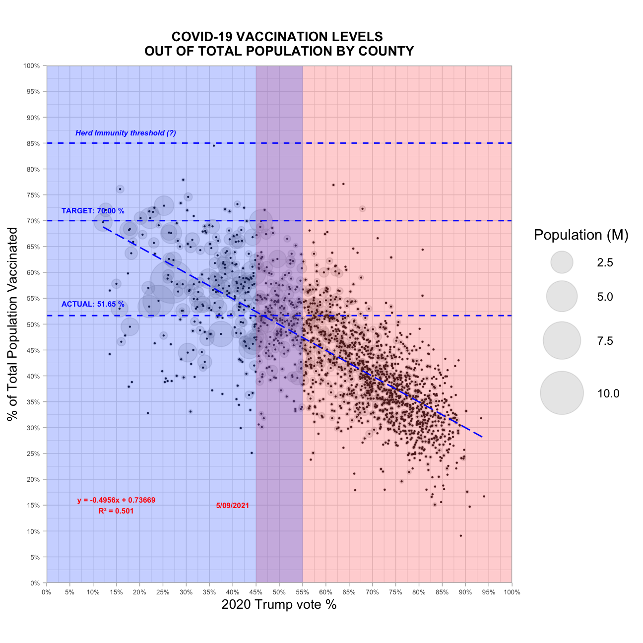
print(summary(lm(vax_complete_pop_pct,formula = series_complete_pop_pct ~ prcOfVote)))##
## Call:
## lm(formula = series_complete_pop_pct ~ prcOfVote, data = vax_complete_pop_pct)
##
## Residuals:
## Min 1Q Median 3Q Max
## -31.19 -4.50 0.09 4.60 34.06
##
## Coefficients:
## Estimate Std. Error t value Pr(>|t|)
## (Intercept) 74.8328 0.7748 96.6 <2e-16 ***
## prcOfVote -0.4985 0.0118 -42.4 <2e-16 ***
## ---
## Signif. codes: 0 '***' 0.001 '**' 0.01 '*' 0.05 '.' 0.1 ' ' 1
##
## Residual standard error: 7.68 on 1721 degrees of freedom
## Multiple R-squared: 0.51, Adjusted R-squared: 0.51
## F-statistic: 1.79e+03 on 1 and 1721 DF, p-value: <2e-16sprintf("Percentage of the total population vaccinated: %0.2f ",sum(vax_complete_pop_pct$series_complete_pop_pct*vax_complete_pop_pct$pop)/sum(vax_complete_pop_pct$pop))## [1] "Percentage of the total population vaccinated: 52.72 "Kázmér Nagy-Betegh
I love to work on challanges that intersection technology and business.